We are excited to announce new capabilities which are apart of time-series forecasting in Azure Machine Learning service. We launched preview of forecasting in December 2018, and we have been excited with the strong customer interest. We listened to our customers and appreciate all the feedback. Your responses helped us reach this milestone. Thank you.

Building forecasts is an integral part of any business, whether it’s revenue, inventory, sales, or customer demand. Building machine learning models is time-consuming and complex with many factors to consider, such as iterating through algorithms, tuning your hyperparameters and feature engineering. These choices multiply with time series data, with additional considerations of trends, seasonality, holidays and effectively splitting training data.
Forecasting within automated machine learning (ML) now includes new capabilities that improve the accuracy and performance of our recommended models:
- New forecast function
- Rolling-origin cross validation
- Configurable Lags
- Rolling window aggregate features
- Holiday detection and featurization
Expanded forecast function
We are introducing a new way to retrieve prediction values for the forecast task type. When dealing with time series data, several distinct scenarios arise at prediction time that require more careful consideration. For example, are you able to re-train the model for each forecast? Do you have the forecast drivers for the future? How can you forecast when you have a gap in historical data? The new forecast function can handle all these scenarios.
Let’s take a closer look at common configurations of train and prediction data scenarios, when using the new forecasting function. For automated ML the forecast origin is defined as the point when the prediction of forecast values should begin. The forecast horizon is how far out the prediction should go into the future.
In many cases training and prediction do not have any gaps in time. This is the ideal because the model is trained on the freshest available data. We recommend you set your forecast this way if your prediction interval allows time to retrain, for example in more fixed data situations such as financial forecasts rate or supply chain applications using historical revenue or known order volumes.
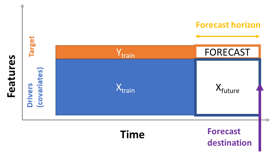
When forecasting you may know future values ahead of time. These values act as contextual information that can greatly improve the accuracy of the forecast. For example, the price of a grocery item is known weeks in advance, which strongly influences the “sales” target variable. Another example is when you are running what-if analyses, experimenting with future values of drivers like foreign exchange rates. In these scenarios the forecast interface lets you specify forecast drivers describing time periods for which you want the forecasts (Xfuture).
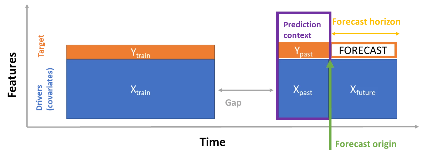
If train and prediction data have a gap in time, the trained model becomes stale. For example, in high-frequency applications like IoT it is impractical to retrain the model constantly, due to high velocity of change from sensors with dependencies on other devices or external factors e.g. weather. You can provide prediction context with recent values of the target (ypast) and the drivers (Xpast) to improve the forecast. The forecast function will gracefully handle the gap, imputing values from training and prediction context where necessary.
In other scenarios, such as sales, revenue, or customer retention, you may not have contextual information available for future time periods. In these cases, the forecast function supports making zero-assumption forecasts out to a “destination” time. The forecast destination is the end point of the forecast horizon. The model maximum horizon is the number of periods the model was trained to forecast and may limit the forecast horizon length.

The forecast model enriches the input data (e.g. adds holiday features) and imputes missing values. The enriched and imputed data are returned with the forecast.
Notebook examples for sales forecast, bike demand and energy forecast can be found on GitHub.
Rolling-origin cross validation
Cross-validation (CV) is a vital procedure for estimating and reducing out-of-sample error for a model. For time series data we need to ensure training only occurs using values to the past of the test data. Partitioning the data without regard to time does not match how data becomes available in production, and can lead to incorrect estimates of the forecaster’s generalization error.
To ensure correct evaluation, we added rolling-origin cross validation (ROCV) as the standard method to evaluate machine learning models on time series data. It divides the series into training and validation data using an origin time point. Sliding the origin in time generates the cross-validation folds.
As an example, when we do not use ROCV, consider a hypothetical time-series containing 40 observations. Suppose the task is to train a model that forecasts the series up-to four time-points into the future. A standard 10-fold cross validation (CV) strategy is shown in the image below. The y-axis in the image delineates the CV folds that will be made while the colors distinguish training points (blue) from validation points (orange). In the 10-fold example below, notice how folds one through nine result in model training on dates future to be included the validation set resulting inaccurate training and validation results.
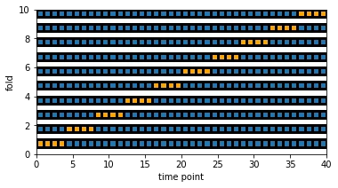
This scenario should be avoided for time-series instead, when we use an ROCV strategy as shown below, we preserve the time series data integrity and eliminate the risk of data leakage.
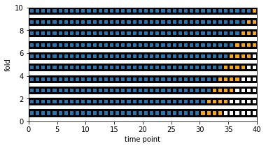
ROCV is used automatically for forecasting. You simply pass the training and validation data together and set the number of cross validation folds. Automated machine learning (ML) will use the time column and grain columns you have defined in your experiment to split the data in a way that respects time horizons. Automated ML will also retrain the selected model on the combined train and validation set to make use of the most recent and thus most informative data, which under the rolling-origin splitting method ends up in the validation set.
Lags and rolling window aggregates
Often the best information a forecaster can have is the recent value of the target. Creating lags and cumulative statistics of the target then increases accuracy of your predictions.
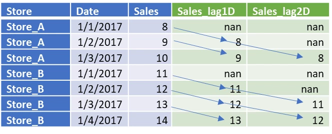
In automated ML, you can now specify target lag as a model feature. Adding lag length identifies how many rows to lag based on your time interval. For example, if you wanted to lag by two units of time, you set the lag length parameter to two.
The table below illustrates how a lag length of two would be treated. Green columns are engineered features with lags of sales by one day and two day. The blue arrows indicate how each of the lags are generated by the training data. Not a number (Nan) are created when sample data does not exist for that lag period.
In addition to the lags, there may be situations where you need to add rolling aggregation of data values as features. For example, when predicting energy demand you might add a rolling window feature of three days to account for thermal changes of heated spaces. The table below shows feature engineering that occurs when window aggregation is applied. Columns for minimum, maximum, and sum are generated on a sliding window of three based on the defined settings. Each row has a new calculated feature, in the case of date January 4, 2017 maximum, minimum, and sum values are calculated using temp values for January 1, 2017, January 2, 2017, and January 3, 2017. This window of “three” shifts along to populate data for the remaining rows.

Generating and using these additional features as extra contextual data helps with the accuracy of the trained model. This is all possible by adding a few parameters to your experiment settings.
Holiday features
For many time series scenarios, holidays have a strong influence on how the modeled system behaves. The time before, during, and after a holiday can modify the series’ patterns, especially in scenarios such as sales and product demand. Automated ML will create additional features as input for model training on daily datasets. Each holiday generates a window over your existing dataset that the learner can assign an effect to. With this update, we will support over 2000 holidays in over 110 countries. To use this feature, simply pass the country code as a part of the time series settings. The example below shows input data in the left table and the right table shows updated dataset with holiday featurization applied. Additional features or columns are generated that add more context when models are trained for improved accuracy.

Get started with time-series forecasting in automated ML
With these new capabilities automated ML increases support more complex forecasting scenarios, provides more control to configure training data using lags and window aggregation and improves accuracy with new holiday featurization and ROCV. Azure Machine Learning aims to enable data scientists of all skill levels to use powerful machine learning technology that simplifies their processes and reduces the time spent training models. Get started by visiting our documentation and let us know what you think – we are committed to make automated ML better for you!
Learn more about the Azure Machine Learning service and get started with a free trial.
