

Advancing enterprise AI: New SAP on Azure announcements from SAP Sapphire 2026
Together, Microsoft and SAP are helping enterprises transform operations, decision-making, and innovation at scale on Azure.
Together, Microsoft and SAP are helping enterprises transform operations, decision-making, and innovation at scale on Azure.

Microsoft and Red Hat show how Azure Red Hat OpenShift powers modernization and production AI with secure, scalable enterprise governance.

As demand for cloud and AI grows, Microsoft is expanding Azure across Europe to deliver scalable, resilient infrastructure that supports innovation, compliance, and performance.

Azure API Management provides a single, Azure-native platform to govern everything from traditional APIs to AI models, tools, and agents.
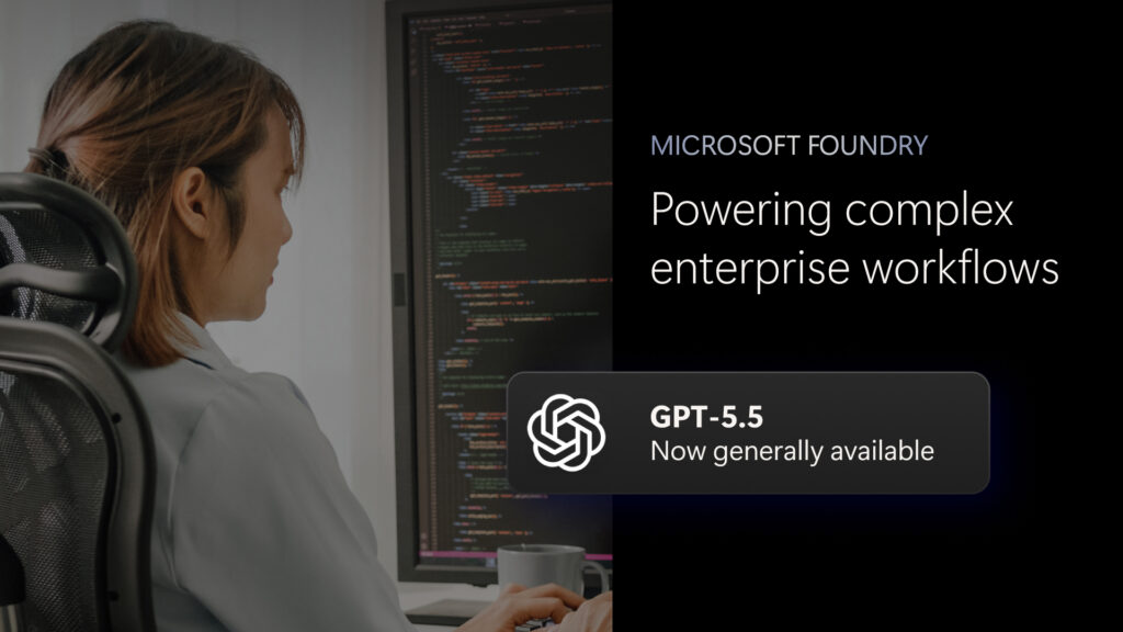
OpenAI’s GPT-5.5 will be generally available in Microsoft Foundry, bringing OpenAI’s latest frontier model to Azure and the enterprise teams building agents for real production work.
Expanded preview access for Microsoft Discovery brings new enterprise-grade, agentic AI capabilities for research and development teams.
Discover how cloud cost optimization adapts in the age of AI, with best practices for managing spend, improving efficiency, and maximizing value.
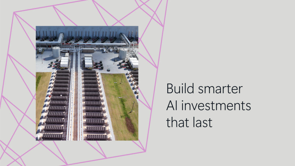
Get practical strategies and best practices to help you plan, design, and manage AI investments for sustainable value and efficiency.

To break the infrastructure bottleneck and shift the industry from ambition to delivery, Microsoft is announcing an AI for nuclear collaboration with NVIDIA, to provide end-to-end tools that streamline permitting, accelerate design, and optimize operations across the industry.

We’re bring attendees together to share real experiences and solve challenges side-by-side. Only together can we move into meaningful results.

Microsoft combines accelerated computing with cloud scale engineering to bring advanced AI capabilities to our customers. For years, we’ve worked with NVIDIA to integrate hardware, software and infrastructure to power many of today’s most important AI breakthroughs.

Discover how cloud modernization and agentic AI are accelerating migration across healthcare, financial services, and manufacturing.